Area Problem Revisited
 We have already talked about the area problem and have presented one approach to solve this problem. Here, we are going to demonstrate a different approach.
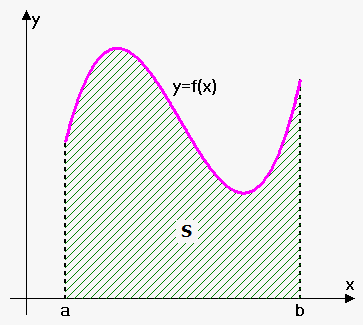
So, suppose that we are given a function $$${f{{\left({x}\right)}}}$$$ that is positive on $$${\left[{a},{b}\right]}$$$ and we want to find the area $$${S}$$$ under the curve. It is not so easy to find the area of a region with curved sides. So, we will start from rectangle approximation.
To get a better understanding, let's start with an example.
Example. Use rectangles to estimate the area under the parabola $$${f{{\left({x}\right)}}}={{x}}^{{2}}$$$ from $$$0$$$ to $$$1$$$.
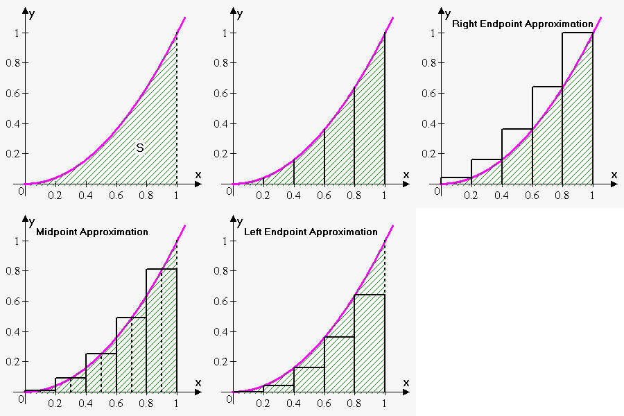
Let's divide the area $$${S}$$$ into five strips. We can approximate the area of each strip by the area of the rectangle whose base is the same as the base of the strip and whose height is the same as the right edge of the strip (the value of the function at the rightmost point of the strip).
Since we divided the interval $$${\left[{0},{1}\right]}$$$ into five strips, the length of the base of each strip is $$$\frac{{{1}-{0}}}{{5}}={0.2}$$$.
So, we have the following five subintervals: $$${\left[{0},{0.2}\right]}$$$, $$${\left[{0.2},{0.4}\right]}$$$, $$${\left[{0.4},{0.6}\right]}$$$, $$${\left[{0.6},{0.8}\right]}$$$, $$${\left[{0.8},{1}\right]}$$$.
As already stated above, the length of the base of each strip is $$$0.2$$$. This is also the base of each rectangle.
Now, let's see what the area of each rectangle is. Recall that the height is the value of a function at the right endpoint.
First rectangle: the height is $$${{0.2}}^{{2}}$$$; so, the area is $$${S}_{{1}}={0.2}\cdot{{0.2}}^{{2}}.$$$
Second rectangle: the height is $$${{0.4}}^{{2}}$$$; so, the area is $$${S}_{{2}}={0.2}\cdot{{0.4}}^{{2}}$$$.
Third rectangle: the height is $$${{0.6}}^{{2}}$$$; so, the area is $$${S}_{{3}}={0.2}\cdot{{0.6}}^{{2}}$$$.
Fourth rectangle: the height is $$${{0.8}}^{{2}}$$$; so, the area is $$${S}_{{4}}={0.2}\cdot{{0.8}}^{{2}}$$$.
Fifth rectangle: the height is $$${{1}}^{{2}}$$$; so, the area is $$${S}_{{5}}={0.2}\cdot{{1}}^{{2}}$$$.
The sum of the areas of these approximating rectangles is $$${R}_{{5}}={0.2}\cdot{{0.2}}^{{2}}+{0.2}\cdot{{0.4}}^{{2}}+{0.2}\cdot{{0.6}}^{{2}}+{0.2}\cdot{{0.8}}^{{2}}+{0.2}\cdot{{1}}^{{2}}=\frac{{11}}{{25}}={0.44}$$$.
As can be seen, $$${R}_{{5}}$$$ is greater than the area $$${S}$$$; so, $$${S}<{0.44}$$$.
Instead of using the right endpoints, we could use the smaller rectangles whose heights are the values at the left-hand endpoints of the subintervals (the leftmost rectangle collapsed because its height is $$$0$$$).
Let's see what the area of each rectangle is. Recall that the height is the value of a function at the left endpoint.
First rectangle: the height is $$${{0}}^{{2}}$$$; so, the area is $$${S}_{{1}}={0.2}\cdot{{0}}^{{2}}$$$.
Second rectangle: the height is $$${{0.2}}^{{2}}$$$; so, the area is $$${S}_{{2}}={0.2}\cdot{{0.2}}^{{2}}$$$.
Third rectangle: the height is $$${{0.4}}^{{2}}$$$; so, the area is $$${S}_{{3}}={0.2}\cdot{{0.4}}^{{2}}$$$.
Fourth rectangle: the height is $$${{0.6}}^{{2}}$$$; so, the area is $$${S}_{{4}}={0.2}\cdot{{0.6}}^{{2}}$$$.
Fifth rectangle: the height is $$${{0.8}}^{{2}}$$$; so, the area is $$${S}_{{5}}={0.2}\cdot{{0.8}}^{{2}}$$$.
The sum of the areas of these approximating rectangles is $$${L}_{{5}}={0.2}\cdot{{0}}^{{2}}+{0.2}\cdot{{0.2}}^{{2}}+{0.2}\cdot{{0.4}}^{{2}}+{0.2}\cdot{{0.6}}^{{2}}+{0.2}\cdot{{0.8}}^{{2}}=\frac{{6}}{{25}}={0.24}$$$.
As can be seen, the area $$${S}$$$ is larger than $$${L}_{{5}}$$$; so, $$${0.24}<{S}<{0.44}$$$.
Finally, we can take the height of the rectangles to be the value of the function at the midpoint of the interval.
The corresponding approximation is $$${M}_{{5}}={0.2}\cdot{{0.1}}^{{2}}+{0.2}\cdot{{0.3}}^{{2}}+{0.2}\cdot{{0.5}}^{{2}}+{0.2}\cdot{{0.7}}^{{2}}+{0.2}\cdot{{0.9}}^{{2}}=\frac{{33}}{{100}}={0.33}$$$.
Since it is not clear what is greater: $$${S}$$$ or $$${M}_{{5}}$$$, we just write $$${S}\approx{0.33}$$$.
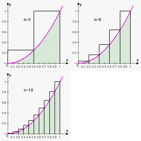
What will be if we increase the number of strips? Clearly, the greater the number of strips, the  better approximation we obtain.
So, let's see what will be if we approximate the area by a very large number of rectangles.
Suppose that we have divided the area into $$${n}$$$ strips. Then, the length of the base of each strip is $$$\frac{{{1}-{0}}}{{n}}=\frac{{1}}{{n}}$$$.
Let's use right-endpoint approximation. In this case, the height of the $$$i$$$-th rectangle is $$${{\left(\frac{{1}}{{i}}\right)}}^{{2}}$$$, and the area of the $$$i$$$-th rectangle is $$${A}_{{i}}=\frac{{1}}{{n}}\cdot{{\left(\frac{{i}}{{n}}\right)}}^{{2}}$$$.
Summing the areas of the rectangles will give the approximate area:
$$${S}_{{n}}=\frac{{1}}{{n}}\cdot{{\left(\frac{{1}}{{n}}\right)}}^{{2}}+\frac{{1}}{{n}}\cdot{{\left(\frac{{2}}{{n}}\right)}}^{{2}}+\ldots+\frac{{1}}{{n}}\cdot{{\left(\frac{{n}}{{n}}\right)}}^{{2}}={\sum_{{{i}={1}}}^{{n}}}\frac{{1}}{{n}}{{\left(\frac{{i}}{{n}}\right)}}^{{2}}=\frac{{1}}{{{n}}^{{3}}}{\sum_{{{i}={1}}}^{{n}}}{{i}}^{{2}}$$$.
To rewrite this formula, we need the following formula: $$${\sum_{{{i}={1}}}^{{n}}}{{i}}^{{2}}=\frac{{{n}{\left({n}+{1}\right)}{\left({2}{n}+{1}\right)}}}{{6}}$$$.
So, we can write that $$${S}_{{n}}=\frac{{1}}{{{n}}^{{3}}}\frac{{{n}{\left({n}+{1}\right)}{\left({2}{n}+{1}\right)}}}{{6}}=\frac{{{\left({n}+{1}\right)}{\left({2}{n}+{1}\right)}}}{{{6}{{n}}^{{2}}}}=\frac{{{2}{{n}}^{{2}}+{3}{n}+{1}}}{{{6}{{n}}^{{2}}}}=\frac{{1}}{{3}}+\frac{{1}}{{{2}{n}}}+\frac{{1}}{{{6}{{n}}^{{2}}}}.$$$
If we now make $$${n}$$$ very large, we will find the required area $$${S}$$$: $$${S}=\lim_{{{n}\to\infty}}{S}_{{n}}=\lim_{{{n}\to\infty}}{\left(\frac{{1}}{{3}}+\frac{{1}}{{{2}{n}}}+\frac{{1}}{{{6}{{n}}^{{2}}}}\right)}=\frac{{1}}{{3}}$$$ (this is just the limit of the sequence).
So, $$${S}=\frac{{1}}{{3}}$$$.
Let's apply this idea to our initial problem – the problem of finding the area under the continuous curve $$${y}={f{{\left({x}\right)}}}$$$ on the interval $$${\left[{a},{b}\right]}$$$.
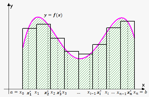
We start by dividing $$${S}$$$ into $$${n}$$$ strips $$${S}_{{1}}$$$, $$${S}_{{2}}$$$,...,$$${S}_{{n}}$$$ of equal width.
The widht of the interval $$${\left[{a},{b}\right]}$$$ is $$${b}-{a}$$$; so, the width of each of the $$${n}$$$ strips is $$$\Delta{x}=\frac{{{b}-{a}}}{{n}}$$$.
These strips divide the interval $$${\left[{a},{b}\right]}$$$ into $$${n}$$$ strips:
$$${\left[{x}_{{0}},{x}_{{1}}\right]},{\left[{x}_{{1}},{x}_{{2}}\right]},\ldots,{\left[{x}_{{{n}-{1}}},{x}_{{n}}\right]}$$$, where $$${x}_{{0}}={a}$$$ and $$${x}_{{n}}={b}$$$.
In fact, if we let $$${n}\to\infty$$$, then it doesn't matter what height of the rectangle to choose: $$${h}_{{i}}={a}+{i}\Delta{x}$$$ (right endpoint), $$${h}_{{i}}={a}+{\left({i}-{1}\right)}\Delta{x}$$$ (left endpoint), or $$${h}_{{i}}={a}+{i}\Delta{x}-\Delta\frac{{x}}{{2}}$$$ (midpoint). In fact, we can choose any sample point $$${{x}_{{i}}^{\star}}$$$ from the interval $$${\left[{x}_{{{i}-{1}}},{x}_{{i}}\right]}$$$.
In this case, the area of the $$$i$$$-th rectangle is $$${A}_{{i}}={f{{\left({{x}_{{i}}^{\star}}\right)}}}\Delta{x}$$$.
Now, the area $$${S}$$$ can be approximated by summing the areas of the $$${n}$$$ rectangles: $$${S}_{{n}}={f{{\left({{x}_{{1}}^{\star}}\right)}}}\Delta{x}+{f{{\left({{x}_{{2}}^{\star}}\right)}}}\Delta{x}+\ldots+{f{{\left({{x}_{{n}}^{\star}}\right)}}}\Delta{x}={\sum_{{{i}={1}}}^{{n}}}{f{{\left({{x}_{{i}}^{\star}}\right)}}}\Delta{x}$$$.
This approximation becomes better and better as $$${n}\to\infty$$$.
Fact. The area $$${S}$$$ of the region that lies under the graph of a continuous function $$${f{}}$$$ is the limit of the sum of the areas of the approximating rectangles: $$${S}=\lim_{{{n}\to\infty}}{S}_{{n}}=\lim_{{{n}\to\infty}}{\sum_{{{i}={1}}}^{{n}}}{f{{\left({{x}_{{i}}^{\star}}\right)}}}\Delta{x}$$$.
It can be proved that the above limit always exists, since we are assuming that $$${f{}}$$$ is continuous.
